9. VE closed loop

Version 1.1Software: FuelTech Vision 3.0Firmware: 00.03.00.54Products: FT700, FT470, VisionFT2026-10-14

The VE closed loop compares the lambda measured by the O2 sensor with the target and corrects the volumetric efficiency that the model uses, before the fuel is calculated.

It does not change the VE table and does not act directly on the injection time: the correction enters as a factor on the VE from the table, and pressure, injectors and banks already receive the corrected VE.

There are two layers. The Fast correction (STFT) follows the O2 sensor and is the subject of this chapter. The Long term learning (LTFT) stores the correction by map region and is in Self-learning: VE learning (LTFT).

The function is in the Fuel tables > Fuel closed loop (VE) menu (on the VCU screen, the Fuel injection menu) and only appears with the Fuel strategy set to VE Based.

It is off in a new map. To turn it on, right-click the function on the computer or use a long press on the VCU screen. All the function settings, except the on/off switch, can be changed with the engine running.

In VE mode, FuelTech Vision turns off the closed loop of the pulsewidth mode and hides its menu: the two never correct at the same time.

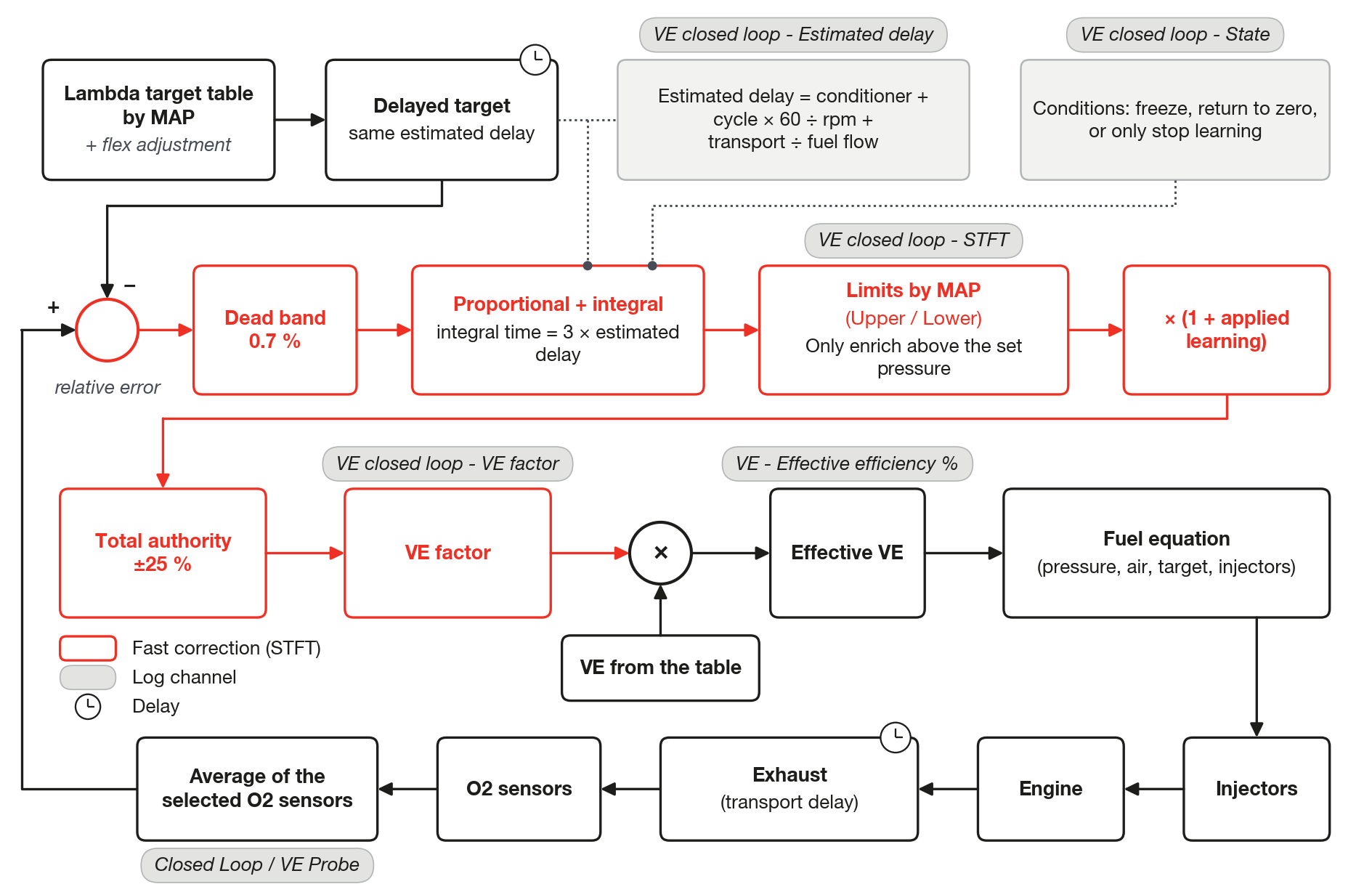
The correction path: delayed target, comparison with the O2 sensor, limits and factor applied to the VE

#What the fast correction corrects

The correction measures the relative error between the O2 sensor and the lambda target:

error = (measured lambda - delayed target) ÷ delayed target
positive error = lean mixture = the correction adds fuel

The delayed target is the lambda target shifted in time by the O2 sensor delay, explained in the section O2 sensor transport delay, further on.

The target comes from the Lambda target table by MAP, plus the flex adjustment when it is active.

Enrichments in % (warm-up, gear, air conditioning, electric fan, custom functions) increase the fuel but do not change the target: with the loop acting, an enrichment that stays on at steady state appears as error, the correction removes it up to its limit and the learning stores what it removed. See Steady-state enrichment with the loop on, in Enrichments and compensations in VE mode.

Errors smaller than 0.7% are treated as zero, so the correction does not chase the O2 sensor noise. This is the default 0.007 of the Lambda error dead band.

#When the correction acts

The loop only corrects with the engine at steady state and with a reliable O2 sensor. Each condition does one of three things: freezes the correction, which stops correcting; takes the correction back to zero; or only prevents learning, and the correction continues. On the VE learning (LTFT) screen, the Conditions (gates) list shows each condition in green (free), red (freezes the correction or takes it to zero) or yellow (only blocks learning).

Condition	Factory default	What happens to the fast correction
Engine stopped, start, post-start and the Time after start to begin	15 s	Returns to zero with a time constant of 1 s
Engine below the Minimum engine temperature, or engine temperature sensor failure	70 °C	Freezes the value
RPM outside the range between Minimum RPM and Maximum RPM	500 to 8000 rpm	Below the minimum, returns to zero; above the maximum, freezes the value
Invalid O2 sensor (no reading or below 0.2) or stuck	fixed	Drops 10 percentage points per second until zero
O2 sensor in the average still warming up	fixed	Freezes the value; if the reading is invalid, the line above applies
Fuel cut: injection cut, deceleration cut or gear change cut	2.0 s	Freezes; starts correcting again at least 2.0 s after the end of the cut (Lockout after fuel cut)
Launch, anti-lag (ALS) or pit limit active (state Launch / ALS / pit limit)	-	Freezes the value
Acceleration fuel enrichment above Minimum acceleration fuel enrichment that freezes the correction	0%	Freezes; below the value, only the learning waits
Bank compensation different from zero, applied by a custom function	-	Freezes while the compensation is different from zero
Transient: TPS changes more than TPS change that defines a transient or MAP more than MAP change that defines a transient	5% and 0.05 bar	Freezes; releases 1 to 2 times (estimated delay + 0.3 s) after TPS and MAP stop changing
Injector at 100% duty cycle in any bank	fixed	Freezes the value
Compression test or factory test mode of the VCU	-	Freezes the value
End of a lockout that freezes or zeroes the correction, except the transient	0.3 s	Freezes for an additional estimated delay + Post-transient lockout margin
VE model sensor failure (MAP, air temperature or fuel pressure), or differential pressure outside the Differential pressure tolerance for learning	10%	Keeps correcting; only the learning stops

The count of the Time after start to begin starts at the end of the post-start, which lasts 8 s by default. With the defaults and a warm engine, the correction starts about 24 s after the start: 8 s of post-start, 15 s of wait and the wait for the end of the lockout (estimated delay + 0.3 s).

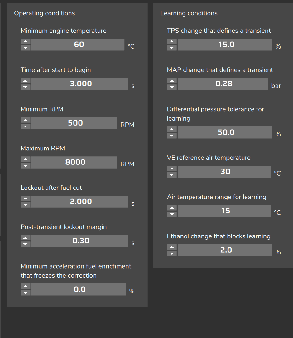
Fuel closed loop (VE), Settings tab: operating conditions and learning conditions (values from a sample map, not the factory defaults).

The other conditions in yellow (air temperature, ethanol, battery, STFT saturated for too long, cell, wait for the STFT to stabilize, moving target, residual acceleration fuel enrichment and saving) also only stop the learning: see Self-learning: VE learning (LTFT).

#Freezing is not forgetting

A frozen correction is only valid near the point where it was learned.

If the engine moves one cell or more of the learning table, the correction slides to the value of that point with a time constant of 1 s: about 63% of the way in 1 s and about 95% in 3 s.

With Rich bias in learning off, which is the default, the value of the new point depends on Apply the learned LTFT: on, it is zero; off, which is also the default, it is the value the learning recorded there, or zero where it has not learned yet.

Example: when coming out of a deceleration with cut, the correction does not carry to the new region the value it had during the deceleration.

The pressure limits remain in force with the correction frozen: see the section How much the correction can change.

#The three ways of returning to zero

Function turned off or map outside VE mode: the correction zeroes immediately and the factor returns to 1.000.
Engine stopped, start, post-start or RPM below the Minimum RPM: returns to zero with a time constant of 1 s.
Invalid or stuck O2 sensor: drops in a straight line, 10 percentage points per second. A correction of 8% takes 0.8 s to reach zero.

The VCU considers the O2 sensor stuck when, in a 5 s window, lambda varies less than 0.002 while the injection pulse of bank A varies more than 10%. It is accepted again as soon as lambda moves 0.002 away from the value where it stopped.

#How the correction is calculated

The correction has two terms, added together.

The proportional term reacts to the error of the moment. With the Proportional gain at the default 0.20, an error of 5% generates 1% of immediate correction.

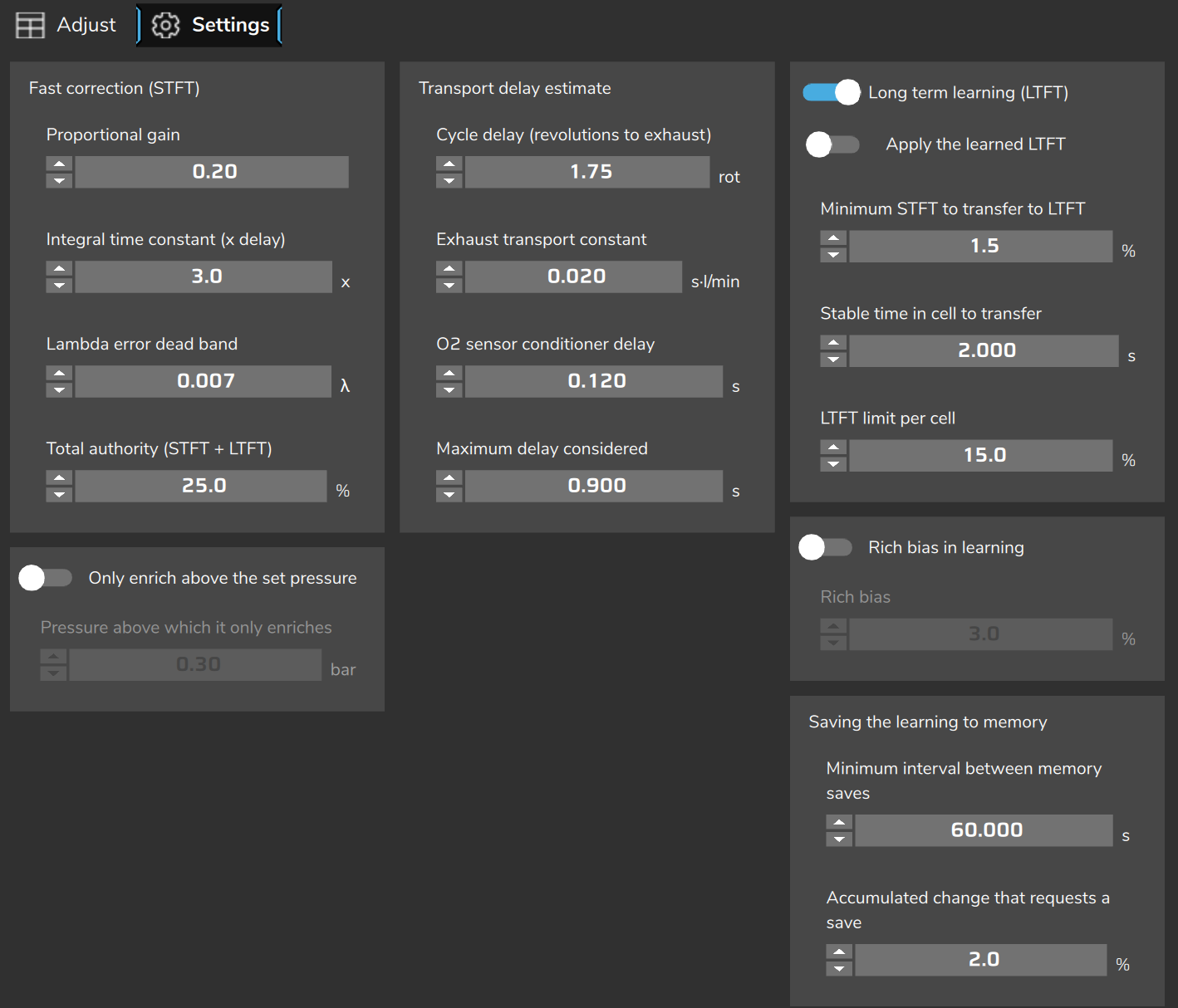
Fuel closed loop (VE), Settings tab: fast correction (STFT), transport delay estimate and long term learning (values from a sample map, not the factory defaults).

The integral term accumulates the error over time and stops growing when the error disappears or when the correction reaches the limit. It is the one that carries the correction that remains.

correction = integral term + proportional gain × error
at each instant, the integral term adds: error × time ÷ (3 × estimated delay)

The 3 in the formula is the default of the Integral time constant (x delay): the integral time is 3 times the estimated delay of the O2 sensor. With a constant error, the integral term adds the value of the error every integral time.

This way the speed adjusts itself to the operating condition: calmer at idle, where the O2 sensor takes longer, and faster under load. There is no gain table to tune.

With the defaults and the fuel flows assumed in the next section, the integral time goes from about 1.8 to 3.7 s at idle, about 0.7 s at cruise and about 0.45 to 0.5 s at high load. With 5% of error, the integral term rises by 1.3 to 2.7% per second at idle and about 10 to 11% per second at high load.

With the correction frozen, only the integral term is kept; the proportional term drops out.

The function help gives an integral time of 2 to 4 times the delay as the stable range.

Recommended practice: if the correction oscillates or is slow, check the estimated delay before touching the gain, because the integral time follows the delay.

#O2 sensor transport delay

Between the injector firing and the O2 sensor seeing the result, time passes: the fuel burns, the gas travels through the exhaust and the O2 sensor conditioner filters the signal.

With the loop on, the VCU estimates this delay continuously, in three terms:

delay = conditioner + cycle × 60 ÷ rpm + transport ÷ fuel flow

O2 sensor conditioner delay (default 0.12 s): fixed term of the O2 sensor signal.
Cycle delay (revolutions to exhaust) (default 1.75 revolutions): matters more at low RPM.
Exhaust transport constant (default 0.020 s·l/min), divided by the fuel flow of the whole engine in liters per minute: matters more at low consumption.

The result never exceeds the Maximum delay considered (default 2.5 s).

With the defaults, the estimate is between 0.6 and 1.3 s at idle at 850 rpm, depending on the engine idle consumption (from 3.3 to 1.2 L/h). At cruise, with 0.3 L/min, it is about 0.2 s and, at high load, at 6000 rpm with 0.9 to 2 L/min, about 0.15 s.

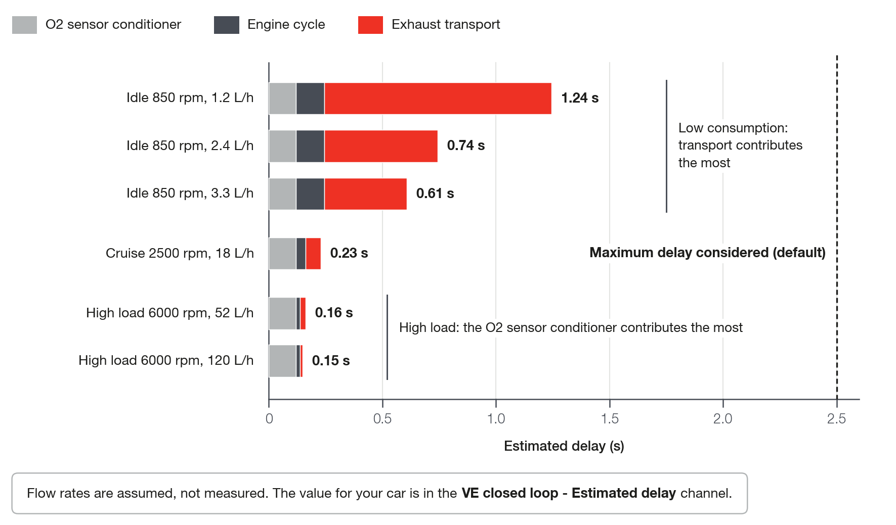
Delay estimate with the defaults: the three terms added up in six operating conditions, with assumed fuel flows

These numbers are an estimate made with assumed flows, not a measurement. The value for your car is in the VE closed loop - Estimated delay channel, in milliseconds.

The channel only shows the calculation with the loop on; with it off, it stays at the Maximum delay considered or at the last calculated value. With the engine stopped or in total fuel cut, such as in deceleration, the flow is zero and the estimate goes to the maximum, which is normal.

#The target is also delayed

The loop does not compare the O2 sensor with the target of the moment: it compares with the target delayed by the same estimated time.

This way, when the engine enters a region with another target, the correction does not chase a change that the O2 sensor has not seen yet.

What remains is a small excursion of the correction, which fades by itself: by calculation, with the default 3, it is estimated at about 12% of the target step.

The same delay defines the waits: the transient window, the wait after a lockout and the time the cell needs to stay stable for the learning.

The Lambda error (O2 sensor vs target) channel compares with the target of the moment, not with the delayed one: see Reading the log: the VE channels.

#Where the O2 sensor is: the transport constant

FuelTech Vision does not know where the O2 sensor is installed. The Exhaust transport constant is how you tell it.

The default 0.020 is a starting point for an O2 sensor at a medium distance from the engine. There is no table of values by position.

The function help gives the direction: increase it for an O2 sensor far from the manifold. An O2 sensor close to the manifold calls for a smaller value. How much, only by measuring.

The calculation divides by the fuel flow. By the preset fuels of FuelTech Vision, ethanol (E100) needs, for the same air, about one third more volume than regular Brazilian gasoline (E27) and about one half more than pure gasoline (E0). Since the time in the exhaust follows the gas flow, and not the fuel flow, it is estimated that, on the same exhaust, the correct constant is larger in the same proportion.

If the delay measured at idle goes over 2.5 s, which can happen with an O2 sensor far away on a small engine, also raise the Maximum delay considered. Otherwise the correct constant has no effect at idle.

#How to check the constant on your car

Warm and stabilized engine at one operating point: first idle, then one or two points of fixed load (dynamometer, or constant RPM and load).
Turn the loop off and record the log at the highest rate, with Closed Loop / VE Probe, VE - O2 closed loop target, RPM and VE total flow.
In the cells around the point, enrich the Lambda target table by MAP by about 10% in one step (for example, from 1.00 to 0.90), hold for 3 to 5 s and go back. Repeat 3 times.
In the log, measure the time between the change of the VE - O2 closed loop target and the instant when the O2 sensor covered two thirds of the way to the new value. Two thirds is a practical criterion for the average delay, which is what the VCU estimates; it does not come from the firmware.
Calculate: constant = (measured time - O2 sensor conditioner delay - Cycle delay (revolutions to exhaust) × 60 ÷ rpm) × flow in L/min.
Save the value, turn the loop on and check that the VE closed loop - Estimated delay is close to the measured time in the same operating conditions.

Hypothetical example: 0.90 s measured at 850 rpm with 0.030 L/min give (0.90 - 0.12 - 0.124) × 0.030 ≈ 0.020.

If the screen shows the flow in L/h, divide by 60; in cc/min, divide by 1000. The unit of the constant is always s·l/min.

With the default 3 in the Integral time constant (x delay), the stable range of the help (2 to 4 times the delay) calls for an estimated delay between two thirds and four thirds of the measured one. Below that the correction tends to oscillate; above, it is slow.

#How much the correction can change

The fast correction has a limit by manifold pressure, in the Fast correction (STFT) limits by MAP table of the Adjust tab, with an Upper and a Lower row.

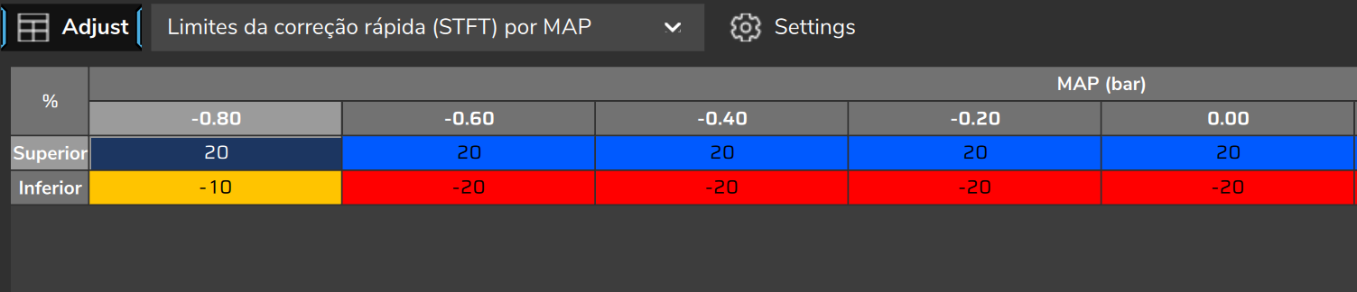
Fast correction (STFT) limits by MAP: Superior and Inferior rows (crop of a sample map, not the factory values).

Factory default, with MAP as gauge pressure, as it appears on the screen. Between the points, the VCU interpolates.

MAP (bar, gauge)	Upper	Lower
−0.8	+10%	−10%
−0.6	+10%	−10%
−0.4	+10%	−10%
−0.2	+10%	−10%
0	+8%	−8%
0.5	+5%	−5%
1.0	+5%	−3%
2.0	+5%	−3%

The fast correction and the applied learning, added together, stay within the Total authority (STFT + LTFT), 25% by default. When the total reaches the limit, the integral term stops growing.

With Apply the learned LTFT off, which is the default, only the fast correction changes the fuel, and what limits it is the table by pressure: the 10% default does not reach the 25%.

A correction stopped at the limit for more than 30 s makes the screen show STFT saturated (VE probably wrong). In this case the error is larger than the limit, and changing the gain does not solve it: in general the VE, the injector flow or the pressure is off, or a steady-state enrichment is on. See Step-by-step tuning method.

#Only enrich at positive pressure

Only enrich above the set pressure is off by default. The function help calls this switch a safety for turbo pressure.

On, above the Pressure above which it only enriches (default 0.30 bar, gauge), the lower limit of the fast correction becomes zero: it can only add fuel. The threshold accepts from −1.0 to 3.0 bar.

This also applies with the correction frozen: a negative correction that came from cruise is zeroed the instant the MAP passes the threshold.

The switch acts only on the fast correction. The applied learning, if Apply the learned LTFT is on, keeps entering the factor, including negative.

#O2 sensors and banks

The loop reads a single lambda: the average of the O2 sensors marked in Sensors and calibration > Wide band O2 sensor > Sensor selection for average value. In the log, this lambda appears as Closed Loop / VE Probe.

The O2 General, the O2 sensors of each cylinder bank (in the list, Left Bank and Right Bank; in the log, O2 Left Bank and O2 Right Bank) and those of each cylinder can be included. In a new map, only the O2 General is marked.

A car with one O2 sensor per cylinder bank must mark these O2 sensors in the selection. Without that, the loop does not see them.

Each O2 sensor only enters the average with a valid reading, from 0.2 up.

With Average value protection on (off by default), readings above lambda 1.090 are left out of the average. If all the O2 sensors in the average go over that, the average becomes invalid and the correction drops to zero instead of enriching.

Only the O2 sensors in the average freeze the loop while they warm up.

The correction is one for the whole engine: the factor multiplies the VE before the fuel is divided among the banks.

If one cylinder bank is rich and the other lean, the loop corrects the average and the imbalance remains.

#How the correction enters the calculation

VE factor    = (1 + applied learning) × (1 + fast correction)
effective VE = VE from the table × VE factor

With the Total authority (STFT + LTFT) of 25%, the factor stays between 0.75 and 1.25.

Example: VE from the table 95%, fast correction +4%, learning not applied. The factor is 1.040 and the effective VE is 98.8%.

The VE table does not change. Taking the correction to the table is your decision, on the VE learning (LTFT) screen: see Self-learning: VE learning (LTFT).

How the fast correction and the applied learning share the factor, with Apply the learned LTFT on or off, is in Self-learning: VE learning (LTFT); the order in which to use the switches on the first run is in From the pulsewidth map to VE.

#What the screen and the log show

The loop state appears as text on the VE learning (LTFT) screen and as a number in the VE closed loop - State log channel. One state appears at a time: when several apply at once, only the one with the highest priority is shown.

The list of states, with the number, the screen text and what happens to the fast correction in each one, is in Reading the log: the VE channels.

In the conditions list, Post-transient lockout lights up after cut, cold engine, enrichment, post-start and other lockouts that freeze or zero the correction. After a transient, the wait appears in the TPS/MAP transient condition itself.

Injectors saturated (staging) means an injector at 100% duty cycle, not the handoff from one bank of injectors to another.

The loop channels (VE closed loop - State, VE closed loop - STFT, VE closed loop - Active LTFT, VE closed loop - VE factor, VE closed loop - Estimated delay, VE - Effective efficiency % and Lambda error (O2 sensor vs target)) are explained in Reading the log: the VE channels.

#Settings of this function

Where each setting is, on the computer and on the VCU screen, with ranges and defaults, is in Parameter reference; how to use the correction to tune the VE, in Step-by-step tuning method.