12. Step-by-step tuning method
This chapter covers the tuning order, the practical rules that avoid the most common mistakes, and how to correct the VE table without losing track of what changed. How each function works is in its own chapter; this chapter holds the method.
#The tuning order
The VE is the last piece and the only one that belongs to the engine. Everything before it is data that you enter; everything after it is correction on top of it.
A wrong input enters the calculation of all the fuel and, if it is corrected in the VE, it hides inside it. That is why the order matters.
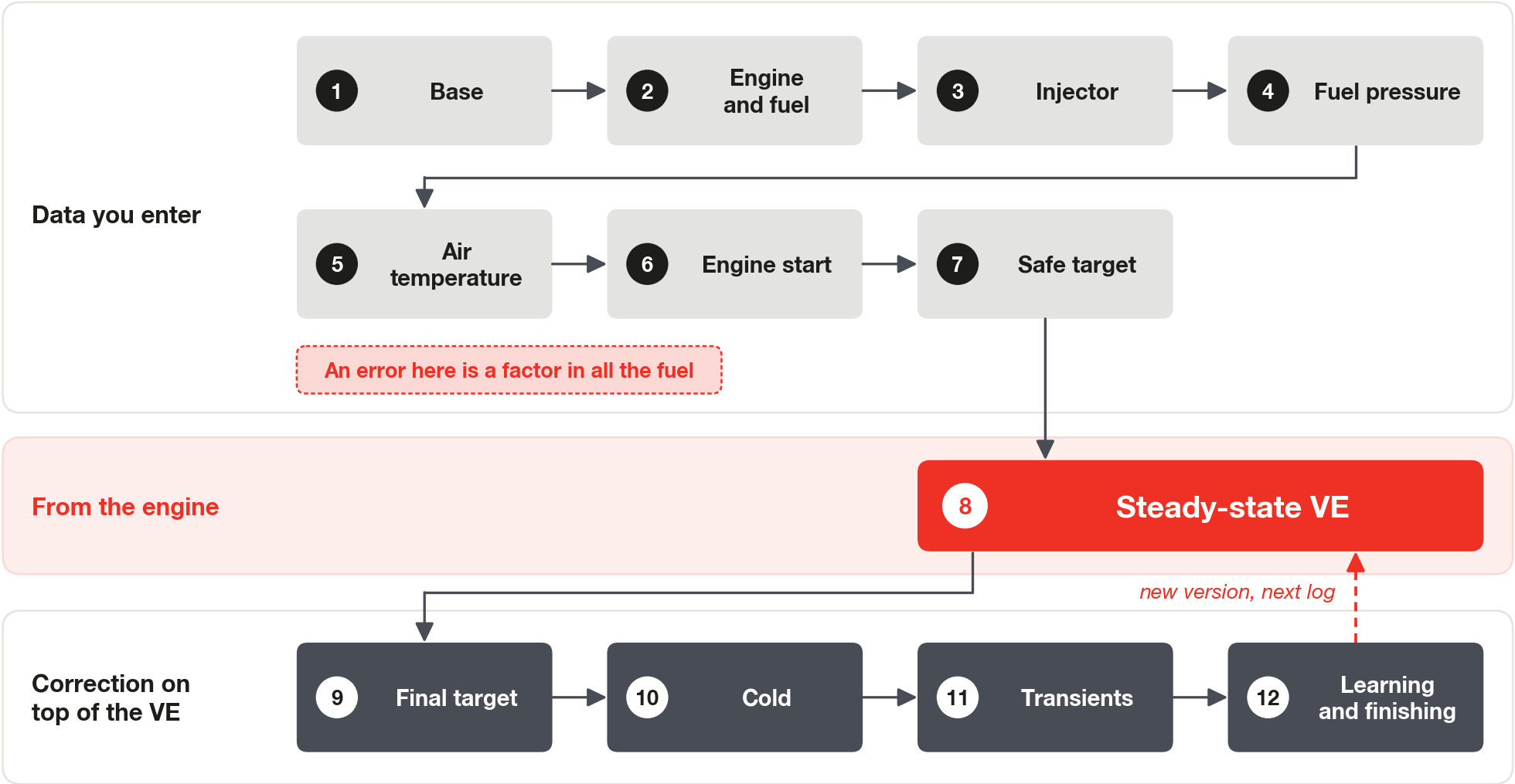
| Step | What to do | Why it comes before the next one |
|---|---|---|
| Base | Note the software and firmware version. Use as the base the map that was in the VCU during the log (Open map from log). | The file on disk may differ from the one that ran; correcting on the wrong base undoes the tune. |
| Engine and fuel | Displacement, number of cylinders and fuel; with flex, the ethanol sensor reading correctly. | They enter as a factor in all the fuel. |
| Injector | Flow rate and rated pressure, from the catalog or measured, deadtime by voltage and pressure, linearization. | A wrong flow rate gives the same error across the whole map; a wrong deadtime gives an error that grows on the short pulse. |
| Fuel pressure | Sensor reading correctly; with no sensor, the sensor option turned off and the failsafe equal to the real differential pressure. | The calculation divides by the square root of the differential pressure: a pressure drop that the VCU does not see becomes VE error. |
| Air temperature | Sensor reading a physical value; only then enabled in the model. | When off, the failsafe applies (25 °C by default); enabled with a wrong reading, the error goes into everything. |
| Engine start | Engine start mode of each bank (the screen calls the banks Primary, Secondary and Tertiary) and the start table. | In Engine start fuel injection table the VE plays no part in cranking. |
| Conservative target | A rich lambda target at load, set before running. | The calculation divides by the target: the measured VE does not change with it, and the rich target puts more fuel at load while the VE is being tuned. |
| Steady-state VE | Cruise cell by cell and full-throttle pulls; measure the required VE per cell, correct in damped steps, check the shape. | This is the step that belongs to the engine. |
| Final target | Lambda target adjusted to the goal (power, temperature). | Changing the target later does not require touching the VE. |
| Cold | Warm-up and post-start. | Below 70 °C (default) the closed loop does not correct; cold is judged with the warm VE already right. |
| Transients | The VE-mode acceleration fuel enrichment. | The cell where the tip-in ends only measures VE in fully settled steady state. |
| Learning and finishing | Delay checked, learning, Diagnostic and Apply to VE; only at the end Apply the learned LTFT. | A correction at the limit points to a wrong base; the learning does not know that the VE changed. |
The closed loop can be on from the first run, with Apply the learned LTFT off. It measures and corrects only within its own limits and does not replace tuning the VE; read the required VE with its correction included (section How to correct, further on).
For the first converted map, follow the first-run procedure in From the pulsewidth map to VE.
#Practical rules
Treat the rules below as recommended practice: each one gives the reason and the mistake it avoids.
#Reading the right data
- Steady state means a steady pedal and MAP; the RPM may rise. The VCU only calls a throttle change above 5% or a MAP change above 0.05 bar a transient, without looking at RPM. A full-throttle pull with the pedal and MAP steady is good data. This avoids discarding all the full-load data and leaving it lean without knowing.
- Align the sensor by the delay, without inventing precision. The sensor sees the combustion after the injection, and the VCU estimates this delay in the channel VE closed loop - Estimated delay, in milliseconds. Use that value and check that the conclusion does not change with 0.1 s more or less. This avoids assigning to one cell the mixture of the previous cell.
- With the closed loop on, the data is the sensor together with the correction. The closed loop has already removed part of the error before the sensor sees it. The right table is the one that leaves VE closed loop - VE factor resting near 1.000 (fast correction near zero and, if the learning is applied, the learning too). This avoids concluding that the error is gone when it was the closed loop that hid it.
- Vary the axis that separates the causes. Between cells of different load the pulse and the MAP move together, and the deadtime is confused with the shape of the table. Hold the MAP row and vary only the RPM: the pulse barely changes, and whatever varies is table shape. This avoids changing the injector flow rate to flatten an error that was one of shape.
- In the cell where the tip-in ends, measure only in fully settled steady state. After the acceleration fuel enrichment returns to zero, its fuel still reaches the sensor with the transport delay, and the fuel that wetted the walls evaporates later. As a rule of thumb, use the samples from 1.5 s, preferably 3 s, after the last trigger. This avoids carrying a leftover of the acceleration fuel enrichment into the table.
#What is not VE
- An equal error across the whole range is flow rate, pressure or fuel. A single factor comes from the flow rate, the injector rated pressure or the stoichiometric AFR; written into the VE, it takes the physical meaning away from the table. This avoids a VE that only closes with the injector entered wrong.
- A high deadtime and a low VE look the same on average. The deadtime is added in milliseconds at the end of the pulse, so its error matters more the shorter the pulse. Separate them by useful time and correct deadtime and VE together, preserving the delivered fuel where it is already right. This avoids a low VE that compensates for a high deadtime, right on the long pulse and wrong at idle.
- A difference between cylinder banks is not corrected in the VE. The VE is a single table, and the closed loop uses one sensor value: the average of the selected sensors. An error only at idle, which goes away with load, points to an air leak on one side; a proportional error across the whole range points to an unbalanced injector or deadtime, which is corrected in the individual cylinder trim. This avoids bending the VE of the whole engine because of one side.
- A sensor with no reading leaves the model blind. Without the reading, the calculation uses fixed values of pressure and air temperature, and the pressure drop under load or the temperature change becomes VE error. A shift of the whole map that follows the temperature of the day points to the air, not to the table. This avoids tuning the VE for the weather of one day.
- Ethanol: check before comparing logs. Without an ethanol sensor the stoichiometric AFR is fixed, and each extra point of ethanol in the fuel changes the stoichiometric AFR by 0.4 to 0.6%, depending on the range. With a sensor, the calculation uses the fuel of the blend, and the learning stops when the ethanol varies by more than 2 points in 10 s. This avoids reading a fuel change as a change in VE.
- A low VE at vacuum can be real. VE is the air drawn in compared with the manifold density. With deep vacuum and an aggressive camshaft, low values at vacuum can be legitimate. Check against fuel consumption before changing anything. This avoids fixing idle by gut feeling and leaving the transition lean.
#How to change the table
- Where you did not measure, leave it rich. Outside the axis the VCU uses the edge value and, inside it, interpolates: a cell with no data is an estimate. Apply to VE does not extrapolate either. This avoids leaning out where nobody measured.
- Correct in damped steps and only with plenty of data. The residual of one log is noisy. Correct the cell that has a lot of data and a repeated sign in at least two logs; a cell whose measurement changes sign waits for the next round. This avoids chasing noise.
- A correction at the limit means a wrong table, not a gain problem. The limit says that the table asks for more than the closed loop can give; a larger gain only reaches the same limit faster. Count the time parked at the limit, not the time with a negative sign. This avoids changing the controller when the problem is the VE.
- On a tip-in, the closed loop carries the correction it had. In a transient the correction is frozen; when the engine moves by one cell, it releases toward the value of the new point with a time constant of 1 s. If the light load is rich, the tip-in starts with a negative correction and leans out the full load for a moment. This avoids leaning out the full load when correcting the light load.
- Remedy for a lean tip-in. Turn on Only enrich above the set pressure, or use a small negative limit in the load columns of Fast correction (STFT) limits by MAP, which applies even with the correction frozen. If you are going to take VE out of the positive-pressure rows, do it in the same map in which you apply one of these remedies. This avoids the VE cut and the negative correction adding up at full load.
- Check the shape before writing. The VCU interpolates, so an absurd value in a row that you never run contaminates the neighbor. As a rule of thumb, the VE does not fall when the MAP rises: a fall in that direction, or a large step between neighboring rows, is suspect and needs checking. When the complaint falls between two rows, adjust the nodes together, not cell by cell. This avoids a correction that closes at the measured point and ruins the neighbor.
- Taking a factor out of the whole map exposes the transition cells. Cells tuned on top of the excess become lean in the same proportion, and the transition from idle to load has no closed loop to save it. Before delivering the map, check the tip-ins of the previous log and correct the transition row at the same time. This avoids trading a rich map for a lean transition.
- Direct injection has no fuel film in the manifold. A misfire or backfire on tip-in, with direct injection, points first to the VE of the transition. A cell with a misfire cannot be measured: work up from the rich side and measure in the next log. This avoids looking in the acceleration fuel enrichment for an error that is in the table.
#Order and control
- VE belongs to the engine; the target is your choice. The fuel is proportional to VE ÷ target. For a richer mixture in a condition, change the lambda target; the percentages serve to replace fuel that does not reach the cylinder (cold wall, transient). This avoids mixing the choice of mixture with a measurement of the engine.
- Zero the steady-state compensations in the range where the closed loop acts. With the closed loop on, warm-up compensation above the closed loop minimum temperature, gear compensation or external-action compensation shows up as error: the closed loop subtracts it up to its limit, and the learning writes that subtraction into the VE. A mixture that is different on purpose goes in the lambda target (see Enrichments and compensations in VE mode). This avoids a VE that turns lean when someone turns the compensation off.
- Cold is judged against the target of the table, with a valid sensor. A sensor at 0.000 is an invalid reading, not a lean mixture. Start the log before turning the key on and judge the start with at least 3 cold starts and a signal other than the sensor (number of attempts, an engine that stalled). This avoids confirming or refuting a start complaint with a single log.
- A car that will not start in VE: look at the start, not the VE. In Engine start fuel injection table, the cranking pulse comes from the engine temperature. In Fuel injection main table, cranking uses the lowest RPM columns of the VE: when rebuilding the grid, do not leave the lowest RPM column with a VE lower than the next one in the atmospheric-pressure rows. This avoids changing the VE for a starting problem.
- Check the delay and inherited parameters before the gain. A map brought from an earlier version may have Exhaust transport constant at 1.5, which pins the delay at the ceiling and makes the closed loop slow. Also check Air temperature range for learning (default 15 °C around the VE reference air temperature, 30 °C by default): with the air sensor reading, the learning only happens with the air inside this window, and a small value blocks it whenever the air leaves it. This avoids changing the gain of a closed loop that was only badly configured.
#Field benchmarks
The numbers in this section are starting points, not a specification. Each one comes with the reason, so you can adjust it to your engine.
#Deadtime above 35% of the pulse
A short pulse is the injector's territory, not the VE's.
The deadtime is added in milliseconds at the end of each pulse. If it is wrong, the error reaches the fuel multiplied by r ÷ (1 − r).
r             = Primary injectors deadtime ÷ Injection time A
useful time   = Injection time A − Primary injectors deadtime
mixture error = deadtime error × r ÷ (1 − r)
r is the fraction of the pulse that is deadtime. Both channels are in the log; the calculation fits in a calculated channel.
| Deadtime in the pulse (r) | Multiplier r ÷ (1 − r) | A 10% deadtime error becomes |
|---|---|---|
| 10% | 0.11 | 1.1% mixture error |
| 20% | 0.25 | 2.5% mixture error |
| 30% | 0.43 | 4.3% mixture error |
| 35% | 0.54 | 5.4% mixture error |
| 50% | 1.00 | 10% mixture error |
| 60% | 1.50 | 15% mixture error |
As a starting point: where the deadtime exceeds 35% of the pulse, do not correct the VE from the sensor.
The 35% is a tolerance choice: it accepts about 5% mixture error for each 10% of error in the deadtime. The less you trust the deadtime table of your injector, the lower this limit should be.
Measure the fraction per cell, in the log. Do not deduce it from the MAP: at light load a whole row can exceed the limit.
In Multipoint, on a piston engine, each pulse carries half of the fuel and the whole deadtime: the short pulse zone is larger than in Sequential.
#Short useful pulse
The injector also stops being linear at a very short pulse, and by how much depends on the injector. Treat as short a useful pulse below 1 to 2 ms, depending on the injector.
By the injector data that FuelTech Vision carries, the nonlinearity disappears above 2 ms. At 0.75 ms it is near 10% on an 80 lb/h high-impedance injector and exceeds 30% on a 520 lb/h or larger, low-impedance injector.
A fixed cutoff at 0.75 ms, therefore, only works as a screening for a small injector.
With a high-impedance injector, the 35% deadtime limit already leaves out practically the whole nonlinear range. With a large low-impedance injector, it does not: fill in the Primary injector linearization table with the manufacturer's short pulse data before tuning idle and light load: the base map wizard leaves it zeroed.
#VE above about 115%
Sanity check: if the VE that the sensor asks for at the best-filling point exceeds about 115%, check the entered injector flow rate, the fuel pressure and the air temperature sensor before accepting the table.
It is not a ceiling. The table accepts up to 300%, and the base map wizard itself never generates a VE above 115%.
The VE of the model absorbs the error of the inputs. A flow rate entered too high shows up as a high VE; an air sensor reading 20 °C hotter than a charge at 40 °C asks for 6.4% more VE.
With alcohol, evaporation can cool the charge below the sensor reading, and a value a little above 115% can be real.
#Two rounds
A map that is far off takes more than one round. With the defaults, Apply to VE moves at most half of what the fast correction reaches: about 5% per round at vacuum. An error larger than the closed loop limit is not learned in full.
So a large error is corrected from the log, by hand, in two rounds or more. Apply to VE is the finishing step.
#How to correct
#Measuring the required VE
The required VE of each cell comes from the log, in a steady-state segment:
Required VE = effective VE × (sensor ÷ target) × (1 + enrichment ÷ 100)Effective VE: channel VE - Effective efficiency %, which already includes the closed loop correction.
Sensor: Closed Loop / VE Probe, read after the delay. Target: VE - O2 closed loop target, in lambda. Enrichment: VE - Total enrichment, in %.
Use only steady-state segments, outside the short pulse zone, outside the tail of the acceleration fuel enrichment and with the enrichment near zero.
How to build this calculation as a channel in the viewer and average a segment is in Reading the log: the VE channels.
#Delivered mixture and table correction
They are two different numbers, and they can have opposite signs:
DELIVERED = sensor ÷ target                          risk to the engine now
BASE      = sensor ÷ target × closed loop factor     how much to change the table
Closed loop factor: channel VE closed loop - VE factor (1.000 means no correction).
Example, with the correction limits widened beyond the default: sensor 0.78, target 0.71, closed loop removing 30% (factor 0.70). DELIVERED = 1.099: the engine is 9.9% lean. BASE = 0.769: the table is 23.1% rich.
#By learning or by hand
The learning measures the error per cell inside the VCU itself. With it connected, Commit to VE carries a fraction of it to the table: 50% by default in Percentage to apply, only in cells with confidence and without extrapolating. The step by step is in Self-learning: VE learning (LTFT).
By hand, from the log, you handle the error larger than the closed loop limit, the transition cells and the positive pressure.
With the defaults, the learning does not learn from 1.0 bar upward and the closed loop corrects only +5/−3% there: full load with a turbo is tuned from the log.
This is the practical sequence:
- Large error first, by hand, in one or more rounds, until the correction leaves the limit.
- Before applying anything, run Diagnostic > Analyze and first correct what is not VE.
- Drive in steady state across the usage ranges and take what is left to the VE with Apply to VE.
- Review the Preview and the shape of the table, save as a new version, send it and record a log before the next change.
#One variable per version
Each map version changes one thing: two changes together make it impossible to know which one acted. Save it in a new file, with the version and what changed in the name, and use the same name inside the map.
Before the log, write down what you will consider accepted and what to check on the first start: nothing is tested until the car's log comes back.
In the next log, check with Open map from log that the map that ran is the one you delivered.
The learning does not know that the VE changed. When changing the VE, axes, injector or pressure, first take what is useful to the VE with Apply to VE, send the map and only then use Clear LTFT. The complete order and the reason are in Self-learning: VE learning (LTFT).
#Limits of the method
- Apply to VE applies a fraction, only where there is confidence, and only separates injector error from VE error when the Diagnostic flags the correlation with 1/PW: always review the preview and record a log.
- Idle with a large injector may not close through the VE: a short pulse belongs to the injector, and that is a result, not a failure of the tune.
- The learning lives in the VCU memory, outside the map file: sending the map to another VCU does not carry the learning.